An Introductory Guide to Multi-Criteria Decision Analysis (MCDA)

What we mean by Multi-Criteria Decision Analysis (MCDA)

MCDA is a way of helping decision-makers rationally choose between multiple options where there are several conflicting objectives. It is often used when:

• there are a mix of criteria that cannot be obviously compared
• there are multiple stakeholder perspectives that affect the decision being made
• other approaches are not suitable

MCDA combines both qualitative and quantitative elements. The qualitative element refers to working with stakeholders to explore their perspectives. The quantitative element refers to using models to represent stakeholder preferences and the performance of different options. These models can then be used to produce useful insights.

Many sources use the term MCDA to refer to any analytical method that supports decision making with multiple objectives or criteria. This guide will concentrate on a subset of methods that might be called ‘classic compensatory MCDA’. These methods use function-based models to reveal an overall numerical rating for each option. This will enable users to see which options are preferred. It is important to be aware that these overall numerical ratings can mean that good performance against some criteria may compensate for poorer performance against other criteria.

You should also be aware that there are other methods that can be used to support decision making with multiple objectives or criteria.

Even with the ‘classic compensatory’ subset, there is considerable variety in the specific methods and techniques that can be used. This guide will concentrate on techniques that provide rigour, without being too complicated.

It is government policy that MCDA can only be used for long list appraisal for decisions that involve public expenditure. Cost Benefit Analysis or Cost Effectiveness Analysis should be used at the shortlisting stage. This policy is set out in paragraphs 4.44 and A1.67 in the Green Book.

If MCDA is only used to assess benefits that cannot be monetised, it should be possible to achieve a high degree of coherence with Cost Benefit Analysis and Cost Effectiveness Analysis.

MCDA is said to be a normative, or prescriptive, approach to decision analysis, rather than a descriptive approach. It indicates what decision should be made if the decision maker is consistent with previously stated preferences. But MCDA rarely captures all the nuances associated with a decision. This means it should be seen as a tool to help decision makers and not as a comprehensive decision-making solution.

The main MCDA steps

Figure 1: Flowchart showing the main MCDA steps

Figure 1 shows the 4 main ‘blocks’ of MCDA activity:

• ‘Structure the problem’
• ‘Establish options and performance’
• ‘Elicit preferences of the decision stakeholders’
• ‘Review the output’

The steps within the ‘structure the problem’ block are:

• identify stakeholders
• understand the decision problem
• identify objectives and criteria
• decide scoring technique by criterion

If your project requires high rigour, you will then need to confirm the criteria scales.

The next block of activity is designed to ‘establish options and performance’. The steps in this block are:

• identify options
• create performance matrix and check for dominance

The next block of activity is designed to ‘elicit preferences of the decision stakeholders’. If your project requires high rigour, you will need to develop component value and functions. If your project requires a lighter touch approach, you will develop a direct rating.

Whether your project requires high rigour or a lighter touch approach, you will then need to weight your criteria.

The next block of activity is designed to ‘review the outputs’. The steps in this block are:

• calculate overall value, or benefit
• examine results, or compare the benefit against the cost
• conduct sensitivity analysis – which may require iteration of steps from the ‘weighting criteria’ phase onwards

Note the cost of options is not considered during the performance matrix or weighting criteria stage, but only at output review stage. See the later section on the treatment of cost in MCDA for a detailed discussion on how option costs should be considered as part of the MCDA process.

These steps and the routes between them are covered in this guide. The guide concentrates on fundamental principles, which means it is not always possible to describe the steps in the same way they appear in this section. We will give an indication of the steps relevant to each section of the guide.

Important messages for commissioners, practitioners, and reviewers

Commissioners

The commissioner is the owner of the question being addressed. They do not need to understand MCDA in detail but they should be satisfied that it is the appropriate approach for the problem.

MCDA quality depends critically upon the selection of suitably experienced practitioners. The commissioner should have sufficient appreciation of MCDA to be confident that the lead practitioner has the necessary skills to select and implement a form of MCDA appropriate to the task.

MCDA approaches sit on a spectrum that ranges from the very simple to the more complex. The simpler approaches have their place, but there is a risk of selecting an overly simple approach for a particular problem, which can lead to inadequate output quality. The consequences of a poor decision should be the main reason for selecting an approach. This is crucial for ensuring that an MCDA is fit for purpose and that its output is defensible from challenge.

The commissioner should also ensure a reviewer is appointed. The reviewer has an important role to play in quality assurance, and they should be independent of the programme from which the problem arises. This is especially important for decisions with high consequences.

Commissioners will typically want to understand timeframe and budget requirements for an MCDA. There is no set answer, as these requirements will depend on:

• the complexity of the problem
• the robustness required
• any constraints

It may be sensible to commission an initial phase of problem exploration and approach selection. After this, conventional project planning techniques should be able to generate time and cost forecasts. If these estimates turn out to be unacceptable, there will be a temptation to simplify the approach, which will invariably reduce rigour. Before the commissioner decides how to proceed, they should consider again:

• the consequences of a poor decision
• the risk of a decision being challenged

MCDA can be applied to:

• discrete-choice problems where the options are mutually-exclusive
• problems concerning portfolios, where multiple options can be selected

The commissioner and the practitioner must be clear about which of these problem types they are dealing with, as there are other considerations needed for portfolio analysis.

Practitioners

The practitioner needs to have the skills of both an analyst and a facilitator.

They need to:

• fully understand and implement the MCDA methods and techniques needed to address the problem
• have access to appropriate tools and experience of how to use them effectively
• be able to facilitate events for colleagues to work together
• be able to elicit information from stakeholders in a controlled manner

This guide provides some information for getting started with MCDA, but a combination of training, further reading and practical experience will be necessary to become a fully competent MCDA practitioner.

Reviewers

The independent reviewer will help the practitioner achieve the appropriate level of rigour. Independent reviewers act to assure quality for the commissioner.

The main source of guidance for UK Government analysis is the Aqua Book. The Aqua Book states that quality analysis needs to:

• be repeatable
• be independent
• be grounded in reality
• be objective
• have understood and managed uncertainty
• address the initial question robustly in the results

The first letters of the words ‘repeatable’, ‘independent’, ‘grounded’, ‘objective’, ‘uncertainty’, and ‘robustly’, create the word ‘rigour’, which provides a useful acronym.

Independent reviewers need to understand of MCDA methods and techniques to a reasonable level to provide an adequate review function. In particular, the reviewer should be familiar with the various pitfalls associated with MCDA. These pitfalls are highlighted in this guide.

Stakeholders and preferences

This section relates to the ‘identify stakeholders’ step in the MCDA process.

The views of various groups of people need to be considered for good decisions to be made within organisations. This means one of the first actions is to identify an adequate set of stakeholders that provide a requisite variety of perspectives relative to the complexity of the problem.

A subset of the stakeholders will need to be appointed as the decision stakeholders. These are the people who will have their preferences formally elicited and represented in the MCDA. This means they will directly influence its output.

The role of the remaining stakeholders is to:

• help establish a shared understanding of the problem context
• provide expert advice

Their preferences are not formally elicited, but they can influence the MCDA output through the decision stakeholders.

Preferences are necessarily subjective, which means precautions need to be taken to ensure a valid outcome of an MCDA. Firstly, the practitioner needs to ensure all stakeholders:

• are engaged with the MCDA approach
• understand their role in the MCDA
• understand how an MCDA has been designed to ensure valid results

The views and preferences of stakeholders are often best captured when they are working together in a workshop setting facilitated by the practitioner. These workshop environments allow:

• perspectives to be shared
• any expressions of undue bias to be challenged or eliminated as far as possible – undue bias could include views that originate from personal aspirations, rather than the aims of the organisation

An experienced practitioner will be skilful in facilitating a constructive debate and applying de-biasing techniques. A particularly useful technique is to question how views that appear unduly biased relate back to relevant strategic objectives.

In the case of government decisions, this means giving due regard to government policy and the national interest. The Green Book mandates that investment decisions relating to public spending should seek to maximise social welfare.

Facilitated workshops that include controlled preference elicitation for input into a MCDA model are known as ‘decision conferences’. Practitioners may need to use techniques for building consensus in these workshops, such as the Delphi method. If stakeholders are unable to reach a consensus, the practitioner may need to consider representing variability of preference in the model and its associated output. You can find out more about this in the ‘uncertainty and risk’ section of this guidance.

A separate group of stakeholders are known as ‘Subject Matter Experts’ (SMEs). Their role is to advise on the performance of options by gathering and reviewing relevant objective evidence. They should not express preferences in this role, although it can be possible for a person to take the roles of both SME and decision stakeholder.

Problem exploration

This section relates to the ‘understand the decision problem’ step in the MCDA process.

Before the quantitative part of an MCDA can start, the problem needs to be thoroughly explored using a range of qualitative techniques. A wide range of problem structuring methods and systems thinking approaches can be used.

Some widely adopted methods include:

• the soft systems methodology
• the strategic choice approach
• strategic options development and analysis

It can be useful for stakeholders to explore the problem together in a workshop environment. This could start by:

• developing a detailed overview to help gain a shared understanding of the problem
• drafting an overall vision to communicate the desired end-state

The technique of laddering involves asking a series of ‘how’ and ‘why’ questions that help identify the fundamental objectives necessary to realise the vision. It can also generate new ideas than may led to new options or decision opportunities.

Sometimes the boundaries of the problem or the effects of external factors are not well understood. In such cases, the development of systems thinking context diagrams or influence diagrams may provide insight.

Figure 2: Example context diagram, or influence diagram, to help with problem exploration

Figure 2 shows an example of a context diagram, or influence diagram, showing how various factors can lead to improved public safety and security. The diagram shows how:

• ‘training quality’ and ‘training accessibility’ both lead directly to ‘better trained staff’, which in turn leads to ‘improved decision making effectiveness’ and then to ‘improved public safety and security’
• ‘information quality’ leads directly to ‘situational awareness’, ‘improved decision making effectiveness’ and then to ‘improved public safety and security’
• ‘external events’ directly influence ‘decision making effectiveness’ and then to ‘improved public safety and security’

If the problem space is affected by uncertainty in the future environment, it may be helpful to use the technique of scenario planning. This can help identify a small number of future scenarios to concentrate on.

Identifying and structuring objectives

Objectives

This section relates to the ‘identify objectives and criteria’ step in the MCDA process.

After adequate problem exploration, there should be a clear, shared understanding of the problem and a vision for the future. You will then be able to create a clearly defined set of objectives, which are the starting point for an MCDA.

MCDA objectives indicate what is desirable, rather than giving specific targets. This is because the MCDA is designed to trade-off achievement between objectives to achieve a good overall balance. Wherever possible, objectives should be expressed as ‘maximise’ and ‘minimise’ statements. If a problem is relatively simple, the list of objectives will be straightforward. But if a problem is more complex, it is best to construct a hierarchy of ‘parent’ and ‘child’ objectives.

Figure 3: An example of a hierarchy of fundamental objectives and criteria

Figure 3 shows a hierarchy of ‘parent and child’ objectives.

Underneath the overall objective of ‘Establish a crisis response service and training centre’ is a series of ‘parent’ objectives such as:

• ‘maximise training capacity’
• ‘minimise environmental impact’
• ‘information systems suitability’
• ‘maximise transport connectivity’

Each ‘parent’ has under it a number of ‘child’ objectives which represent the different cases where the ‘parent’ objective applies, rather than the ways the objective could be achieved.

For example, the parent objective of ‘maximise training capacity’ in the diagram has child objectives that relate to indoor and outdoor training capacity, while the ‘information systems suitability’ parent has ‘maximise system performance’ and ‘maximise technology maturity’. The ‘maximise transport connectivity’ parent has ‘road’, ‘rail’ and ‘air’ as child objectives.

Under each child objective is a unit of measurement that can be used for metrics. For example, training capacity floor area used, or system throughput in terms of calls per hour for maximising system performance.

Note that minimising costs is treated entirely separately to benefits in this diagram.

It is important that the objectives are fundamental objectives to ensure all options can be fairly compared. This means they relate to what is needed, rather than how to achieve it.

So, in a hierarchy, the ‘child’ objectives represent the different cases where the ‘parent’ objective applies, rather than the ways the objective could be achieved. For example, the parent objective of ‘maximise training capacity’ in Figure 3 could have child objectives that relate to indoor and outdoor training capacity, but it should not have ‘maximise number of trainers’. This is because maximising the number of trainers may be only one of several ways of increasing training capacity.

Criteria

This section relates to the following steps in the MCDA process:

• • decide scoring technique by criterion
  • confirm criteria scales

Criteria are measures that indicate progress against objectives. For example, ‘system throughput, or calls per hour’ might be a criterion associated with an objective to ‘maximise system performance’ for a response service.

In MCDA, criteria are vital to help compare options. The more thoroughly the criteria are defined, the better they will be understood. This will also improve the overall quality of output.

Ideally, a scale of measurement should be attached to each criterion. This may be a continuous scale using a direct natural measure, for example, calls per hour. For other criteria, a multi-point discrete scale, or constructed scale, may be used and could be either:

• pre-defined – such as the Technology Readiness Levels for technology maturity
• bespoke for a particular criterion

Some sources use the term ‘attribute’ rather than criterion, especially when there is an associated scale of measurement.

A criterion scale can run in reverse, so that a higher numerical level indicates a criterion that is less desirable. For example, for the ‘maximise transport connectivity’ example, we might use the proxy measure of ‘distance to trunk road’ for the criterion. A greater distance from a trunk road would be less desirable in this context.

All criteria will have a range-of-interest. If it is difficult to establish a complete scale, you should try to at least describe the upper and lower limits to set the range, even if you cannot specify the intermediate points of the scale.

The least rigorous approach is to only describe the criterion itself, without defining any levels. This is acceptable for ‘light touch’ MCDA using direct rating. But there is a risk that people may interpret the criterion and range-of-interest differently.

When the objectives are organised in a hierarchy, criteria only need to be defined for the sub-objectives at the tips of hierarchy. This is because progress against any of the higher level objectives will be the combined effect of progress against its sub-objectives. You can see this in Figure 3.

Options identification and performance assessment

Identifying options

This section relates to the ‘identify options’ step in the MCDA process.

The work to identify options is rarely a single step process. Sometimes options will be defined before an MCDA begins. Sometimes they emerge as the MCDA is designed and the analysis is used to refine them iteratively.

Occasionally, options are not addressed until after the MCDA model has been fully established, including the assessment of weights. This could be part of a deliberate strategy to concentrate on value and benefit. This will also happen when MCDA is used to define a tender evaluation scheme.

In the public sector, options may range from broad policies, such as new environmental priorities for the transport sector, through to the choice of particular lines of routes for roads, or the selection of individual projects to improve water quality.

Performance Assessment

This section relates to the ‘create performance matrix and check for dominance’ step in the MCDA process.

Performance refers to the level that an option achieves against each criterion, with reference to its scale of measurement. As far as possible, this should be based on objective evidence. If this evidence is not available, you should ask for the judgment of Subject Matter Experts. You should not rely on the judgement of decision stakeholders.

You should document performance data in a performance matrix.

Figure 4: An example performance matrix

The table in Figure 4 shows the score for each option for each criterion. That is, it shows the level that an option achieves against each criterion, with reference to its scale of measurement.

If you have criteria without defined scales or available objective evidence, you can add entries in the performance matrix using a preference score that comes from a direct rating. This is shown by the ‘Environmental impact avoidance’ in the performance matrix diagram. You should be aware that these entries will reflect both:

• an objective level of performance
• the strength-of-preference (desirability) for that performance

Checking for dominance

Once you have completed the performance matrix, it may be possible to eliminate one or more options that are less desirable across all criteria when compared to at least one other option. This is known as eliminating options based on dominance.

For example, in Figure 4, the following options could be eliminated:

• Option A – because it is dominated by Options B, C, D and F
• Option E – because it is dominated by Options C and D

It is important to note that reverse-sense criteria applies to the last three columns of:

• Distance to trunk road
• Distance to rail station
• Distance to airport

This means the higher numerical value in each of these columns indicates they are less desirable.

But it would be premature to eliminate these options. This is because the objective of minimising cost is not represented by the MCDA criteria. This will be the case for many MCDA applications, including Portfolio cases. We will cover this in more detail when we look at the treatment of cost in MCDA.

If the issue of cost does not apply, then dominated options can be eliminated. In theory, this could mean that only one option remains. If this happens, the MCDA should end at this point. In practice, a single dominating option would usually have been identified at an earlier stage and an MCDA would not have been commissioned at all.

The Value Model

This section relates to the ‘calculate overall value or benefit’ step in the MCDA process.

The Value Model is a way of representing the stakeholders’ preferences in a quantifiable way. An Overall Value Function is central to a Value Model and will often be an implementation of a linear additive model in the form: “V= (v1 x w1) + (v2 x w2) + (v3 x w3) + …”.

The terms that begin with “v”, such as “v1” and “v2”, are the measures of Component Value or the Preference Scores associated with each criterion. These terms indicate the strength-of-preference that the decision stakeholders have for a criterion, depending on its performance. This means they indicate the relative extent to which an option is expected to progress the corresponding objective. An interval scale with arbitrary limits is used. The scale will typically run from 0 to 100.

The terms that begin with “w”, such as “w1” and “w2”, are the weights of each criterion. They indicate the relative strength-of-preference of the criteria compared to each other. They are normalised so they are in the range 0 to 1 and give a combined total of 1.

The term “V” is the calculated Overall Value. It reveals the overall strength-of-preference for a given option. It will also be on an interval scale with the same limits as Component Value, meaning that the scale usually runs from 0 to 100. If you are communicating the output of an MCDA to a wider audience, it is often helpful to refer to Overall Value as Overall Benefit.

Eliciting strength-of-preference

It is generally recognised that asking people to directly provide ratings of their strength-of-preference between a set of alternatives can give responses that have limited repeatability. Various techniques have been developed to address this issue that involve asking supplementary or alternative questions. These techniques can be applied to both the assessment of component value and of weights.

The easiest technique is known as ‘ranking/rating’. This technique involves asking decision stakeholders to provide order-of-preference, or ‘rankings’, as a lead-in to strength-of-preference, or ‘ratings’ questions. Order-of-preference responses tend to be highly repeatable.

Some more sophisticated techniques have also been developed, such as some discrete pairwise comparison named methods. These methods avoid the need for stakeholders to provide numerical ratings at all. Instead, stakeholders select from a pre-defined set of comparative preference statements, such as:

• ‘equal preference’
• ‘moderate preference’
• ‘strong preference’

The numerical strength-of-preference is then derived from these using an associated tool.

As all possible pairs of options or criteria can be compared, this can provide an excess number of responses. The tool can examine this redundancy to determine the consistency of the assessments made.

It is important to be aware that these techniques can be:

• less transparent, in terms of allowing the derived ratings to be explained
• more time consuming

Mutual Preferential Independence

It is important to understand that a linear additive model is not the only form of overall value function, but it is the standard form for MCDA. It is only valid when there is Mutual Preferential Independence between the criteria.

Practitioners should have an appreciation of what Mutual Preferential Independence looks like in practice. This is possibly more important than having a formal understanding of the term.

You can detect a lack of Mutual Preferential Independence when stakeholders are reluctant to offer preference judgements on the grounds that ‘it depends’ on another criterion. If this happens, it may be possible to review the selection of objectives and criteria to eliminate it. This will usually be simpler than adopting alternative forms of overall value function, which are beyond the scope of this introductory guide.

Assessing component value

Assessment using component value functions

This section relates to the ‘develop component value functions’ step in the MCDA process.

When criteria scales have been defined, performance and value are explicitly separated. Component value functions are then used to translate between performance and value.

Figure 5: An example component value function

The chart in Figure 5 a chart shows how measurable criterion is translated into a component value. The X axis shows the objective measure. In this case the objective measure is ‘system throughput’, which is measured in calls per hour.

The Y axis shows the component value on a scale of 1 to 100. There is a curved line showing diminishing returns to scale as the throughput increases. For example improving from 80 to 100 calls per hour increases the component value by 50 points, but the increase from 180 to 200 calls per hour only increases the component value by about 10 points.

The first task to develop a component value function is to nominate two points on the criterion scale that define the range-of-interest. The most desirable point on the scale should be set at “v=100” and the least desirable point should be set at “v=0”.

You will then need to establish a few intermediate points. If the criterion has a continuous scale it is recommended that you elicit the points on the criterion scale corresponding to three specific points on the value scale. For example, you should first establish “v=50” as the midpoint between “v=0” and “v=100”. You can then establish:

• “v=25” as the midpoint between “v=0” and “v=50”
• “v=75” as the midpoint between “v=50” and “v=100”

This approach is recommended because it only requires questions about indifference to be asked.

With discrete scales, the value corresponding to each criterion level can be elicited using:

• the ‘rating/ranking’ method
• discrete pairwise comparison between pairs of criterion levels

Once you have established all the points, the component value function can be created by curve-fitting.

The shape of the curve will quite often indicate a case of diminishing returns.

Assessment by direct rating

This section relates to the ‘direct rating’ step in the MCDA process.

Direct rating is used when a criterion scale and corresponding component value function has not been produced. It involves directly eliciting a point on the criterion’s value scale for each option. Direct rating cannot be completed until all options are known.

When applying a ranking/rating technique, decision stakeholders are asked to initially rank the options for that criterion. The lowest option should be ranked at “v=0” and the highest option should be ranked at “v=100”. This will then establish the interval scale for the criterion.

Figure 6: An example of direct rating

Figure 6 has a title of ‘Criterion: Environmental Impact Avoidance’ and is an example of employing direct rating across a series of Options running from A to F. The line is marked with arbitrary values 100 at the top and 0 (zero) at the bottom with intermediate scores of 25, 50 and 75 also indicated.

Option D is marked at the ‘100’ level indicating it is the best option at fulfilling the named criterion.

Option E is marked at the ‘0’ level to indicate it is the worst option.

Options B and C are respectively just above and below the 75-level mark on the line to indicate their performance relative to the best and worst performers.

Similarly, Option F is marked just above the 50 level and Option A just above the 25 level.

Decision stakeholders will then be asked to provide preference scores between those limits for the remaining options. Their scores should be consistent with this scale and the previously stated rankings.

Discrete pairwise comparison techniques can also be used to derive the preference scores.

Direct rating has limited rigour as it conflates assessment of the performance with the strength-of-preference for that performance. In the worst case it can become an unacceptable simple scoring exercise where stakeholders have very little shared understanding of the basis for their scores.

Assessing weights

This section relates to the ‘weight criteria’ step in the MCDA process.

When using a linear additive model, there will be an associated set of weights. These weights must be elicited from the decision stakeholders. The overall output of an MCDA is sensitive to the weights, so you must ensure they are determined in a valid manner.

Inexperienced practitioners often make the mistake of eliciting weightings from stakeholders simply based on the names or descriptions of the criteria and how they perceive their relative importance. The problem with this type of simple weighting is that a criterion may receive a very high weight, simply because it is perceived as very important. For example, this could happen with a criterion related to safety. There may only be a small difference between the ‘worst’ and ‘best’ level when the criterion is examined more closely.

The overall benefit of options

This section relates to the ‘calculate overall value or benefit’ step in the MCDA process.

To calculate the overall benefit of each option you will need to:

• multiply the option’s component value by the corresponding global weight – this will give you the weighted benefit
• total the weighted benefits across all criteria

A stacked chart provides a useful way of visualising the output at this stage.

Figure 9: An example of a stacked chart showing overall benefit of options

Figure 9 shows a stacked chart which provides a useful way of visualising the overall benefit of options with the constituent weighted benefit component contributions of each.

It is important to remember that benefit is measured on an interval scale. That means only the differences in column heights are relevant, not their ratios. So, it would be correct to say that Option C, which is ranked second, is much closer in overall benefit to Option D than it is to Option E. But it would be entirely incorrect to read from the chart that Option B has twice the benefit of Option E.

The nature of an interval scale is well demonstrated by any criterion that has been assessed by direct rating. This is because there will always be one option that appears to have no benefit for that criterion. For example, Option E in Figure 9 appears to have no benefit for ‘Environmental impact avoidance’. In fact, it is only valid to say it has the lowest benefit of all the options for that criterion.

It is also important to remember that these kinds of charts only show rankings based on value, or benefit. They do not show value for money.

The treatment of cost in MCDA

This section relates to ‘cost options’.

We aim to minimise cost in most decision situations, so estimated costs will need to form part of the assessment of the options. This means it is appropriate to include cost minimisation objectives in the objectives hierarchy, although cost sub-objectives should never be treated within the MCDA criteria and weights. Instead, they should be assessed within a separate cost analysis. This applies even when cost estimates are very rough and cost analysis is basic. To support this, the benefits and costs should appear on separate branches of the hierarchy. Different colours or line-styles can be used to reinforce the point that cost factors are not part of the MCDA.

The reason for this separation of benefits and costs is to:

• ensure the validity of cost estimation
• achieve coherence with other recognised forms of appraisal involving costs, such as Cost Benefit Analysis (CBA) and Cost Effectiveness Analysis (CEA)

Cost Benefit Analysis (CBA)

CBA relies on monetising all decision factors as either costs or benefits. If there are no market values, they can be sought through shadow pricing. For example, this can be done by obtaining stated preferences of willingness-to-pay from beneficiaries. For public investments, this often involves samples of citizens. To allow options to be compared, CBA produces output in the forms of:

• Net Present Value (NPV) – this is measured in pounds sterling
• Benefit-Cost Ratio (BCR) – as a dimensionless number

In contrast, MCDA is typically used where there is no clear or obvious way for criteria to be monetised. It normally uses preferences expressed by a relatively small number of informed stakeholders. To maximise coherence between an MCDA and a CBA, it is essential that benefits are not double counted as benefits that can be monetised and benefits that cannot be monetised. Any monetised benefits should be combined with the cost analysis following CBA principles, and not included within the MCDA. It may sometimes be necessary to emphasise that an MCDA is strictly an analysis of non-monetised benefits. Any non-monetised costs should be in the MCDA, but these will normally be expressed as a lesser level of benefit in a particular criterion.

Cost Effectiveness Analysis (CEA)

CEA characterises all options by a non-monetary Measure of Effectiveness (MoE) and their cost. These are then plotted on a scatter chart that shows effectiveness against cost.

To assess the comparative value-for-money of the options you should first consider dominance over effectiveness and cost. Secondly, where possible, options are re-scaled to achieve a common level of effectiveness or cost, to enable direct comparison.

Where such rescaling is not possible, decision stakeholders are consulted to judge whether a certain increase in effectiveness between options is worth the associated increase in cost. This is known as deciding the threshold Incremental Cost Effectiveness Ratio (ICER).

Cost Effectiveness Analysis (CEA) with multiple Measures of Effectiveness (MoEs), or MCDA with separate cost analysis

This section relates to the ‘examine results, or compare the benefit against cost’ step in the MCDA process.

CEA tends to concentrate on a single MoE, or will consider MoEs one at a time. It does not in itself provide a means to analyse the net effect of multiple MoEs.

If you need to analyse the effect of multiple MoEs in your CEA, you can use MCDA principles to understand their combined effect and the benefits they may have. This approach would be effectively equivalent to initiating an MCDA with a separate cost analysis, with the multiple MoEs representing the criteria. No matter how you view this approach, the output will be a chart that plots benefits against cost.

The vertical axis shows the overall benefit from the MCDA, instead of a single MoE in a CEA. The horizontal axis shows overall cost from the cost analysis. This should include any benefits that can be monetised, if present. These benefits should be combined, as appropriate, according to CBA principles. Net Present Cost (NPC) should be used to give positive numbers for the horizontal axis, assuming the costs that can be monetised exceed benefits that can be monetised.

Assessing value for money

To assess value-for-money (VFM) it is necessary to compare options based on incremental increases in benefit and in cost. This is equivalent of applying ICER in CEA. In MCDA, this can be thought of as ‘eliciting a willingness-to-pay, or VFM, function from the stakeholders’. This is similar to an overall value function but with just two criteria and their associated weights:

• overall benefit
• overall cost

This kind of function can be used to create a benefit-cost trade-off heat map.

Figure 10: An example heat map showing the benefit from MCDA against cost

The graph in Figure 10 positions each option from A to F against MCDA benefit on the vertical scale and Cost on the horizontal scale. Here the boundary is formed by Options A, B, C and D. Options E and F are dominated by Option B which has greater benefit and lower cost than either. In terms of cost benefit optimisation, Option B is preferred over Options A, C and D.

In most cases, it will be sufficient to use a linear additive model for this VFM function. This will produce straight contours on the heat map. In some cases, the overall trade-off between benefit and cost may be non-linear. This may be to show a preference for a mid-range solution. With only two criteria in the function, this is relatively straightforward to implement. The contours in Figure 10 are slightly curved, making it non-linear.

It is important to note that the absolute ratio of benefit to cost, or gradient to the origin, should never be used to compare options, just as absolute effectiveness-to-cost ratios should never be used in a CEA. This is because the measure of the benefit, or effectiveness is usually on an interval scale with an arbitrary origin. This means such a ratio is meaningless.

Even if this is not the case, the approach is still invalid as these ratios do not consider the decision stakeholder’s perception of value for money. Instead, this threshold is established arbitrarily, based on the options themselves.

Portfolios

MCDA is sometimes applied to portfolio analysis, in which multiple options can be selected. The problem with this is one of prioritisation and resource allocation. It can be difficult to find the combination of options that provides the highest overall benefit for the budget available.

There are several implications of this problem statement:

• it is impractical to reframe the problem into one of discrete-choice – this is because there are too many potential portfolios to assess
• the requirement for overall benefit to be compared to cost reinforces the need for benefit-cost separation
• since the overall benefit of individual or groups of options needs to be directly comparable to their corresponding costs, the component value measures need to be on a ratio scale, in which zero really means ‘no value’ – defined criteria scales should be used to do this, with the least-desirable limit of the range-of-interest, or “v=0”, set to a ‘worthy of no investment’ level

Identifying a high value-for-money portfolio

The baseline technique for portfolio analysis is to compare the benefit-cost ratios (BCRs) for the options. The highest value-for-money portfolio is identified by ranking the BCRs for each option from highest to lowest and calculating the cumulative cost in that order until the budget is reached.

A plot of cumulative benefit against cumulative cost produces a Pareto frontier. Each point on the frontier represents an optimum portfolio made up of that option and all options to the left. All sub-optimal, or dominated, portfolios will appear below this frontier.

Figure 11: An example chart showing cumulative benefit against cumulative cost for options ranked by increasing BCR

The graph in Figure 11 illustrates the analysis of options as part of an optimal portfolio with a fixed budget limit, which is shown as a solid vertical line on the right-hand side. The highest value-for-money portfolio is identified by comparing the benefit cost ratio (BCR) for each option, then ranking the BCRs from highest to lowest and calculating the cumulative cost in that order until the budget limit is reached.

In this example, Option 6 has the highest BCR, then Option 14, Option 9 and so on, continuing until the lowest BCR Option 4 is added. However, there is insufficient budget to include Option 4 in the recommended portfolio.

This plot of cumulative benefit against cost is called a Pareto Frontier.

BCR ranking is valid in portfolio analysis, unlike in discrete-choice problems, because you do not need to elicit and fix the decision-maker’s willingness-to-pay function. In fact, we are allowing willingness-to-pay for incremental benefit to gradually increase until the budget is allocated.

The BCR ranking approach will only give the best portfolio if the budget aligns with one of the points on the frontier. You can also use an optimisation tool to help you find the highest-value budget constrained portfolio.

Unlike the BCR based technique, an optimiser will iterate to find a solution and will typically be better at allocating the full budget. The optimiser can also include additional constraints in the form of simple dependencies. For example, it can ensure a certain option will be excluded if another specified option is included.

Despite the advantages of the optimiser approach, it is important to remember that no approach to portfolio assessment will be able to represent all complex interrelationships between options. This means it remains important to discuss all issues in a decision conference.

A common problem with portfolio analysis is that the range:resolution of the cost scale exceeds the range:resolution of the benefit scale. For example, if benefit is represented in integers from 0 to 100, the benefit range:resolution is 100:1. If cost is represented in increments of £1,000 from £0 to £10 million, the cost range:resolution is 10,000:1. This will prevent the valid comparison of extremely high cost and extremely low cost options. The simplest way to avoid this issue is to separately assess sub-groups of options that appear in the same broad cost band. You will then be able to decide how to allocate shares of the budget to each sub-group.

Uncertainty and risk

This section relates to the ‘conduct sensitivity analysis’ step in the MCDA process.

There is often uncertainty around how an option will perform against certain criterion. This may be because of uncertainty around the option itself, or because of uncertainty in the external environment that affects the criterion. For example, uncertainty about external factors like climate or threat level may affect certain criteria. We may also find there is variability-of-preference between stakeholders, or that there is uncertainty around cost. Sensitivity analysis can be used to analyse all these issues. It can be applied to both discrete-choice and portfolio problems.

In deterministic sensitivity analysis, any uncertain input parameter can be changed to its highest or lowest extreme. The effect on the overall benefit or value-for-money of an option can then be observed. Input parameters could include performance, environment, weights, or costs.

Figure 12: An example of sensitivity analysis

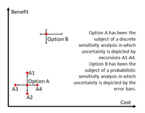
Figure 12 shows a simple graph illustrating the use of sensitivity analysis to reflect uncertainty in how options will perform against criteria. This could be due to external factors or questions about the option itself such as cost or its comparative preference amongst stakeholders.

Sensitivity analysis can be used to analyse all these issues and can be applied to both discrete-choice and portfolio problems.

Option A illustrates deterministic sensitivity analysis in which specific parameters associated with cost or benefit are changed to high/low values and the resulting changes depicted by the ‘excursions’ A1 to A4. These are shown as the extremes around the central case, like points around the centre of a compass. A1 and A2 show the extremes in variability of the benefit of Option A (vertical line) while A3 and A4 show the same for variability of costs (horizontal line).

Option B shows an example of probabilistic sensitivity analysis. This is a more rigorous technique representing uncertain inputs and outputs as probability distributions. This shows the potential extremes in output values in the form of horizontal and vertical error bars around the central point estimate of benefit/cost for Option B.

Initially, inputs should be changed one at time to see which have the greatest effect. A tornado diagram can be used to summarise the findings. After this, combinations of inputs can be changed to assess total risk in the output.

If you have multiple sources of uncertainty, probabilistic sensitivity analysis is a more rigorous technique to use. The technique involves representing uncertain inputs and outputs as probability distributions. This will indicate:

• the extremes in output
• the relative risk of any intermediate point including correlations in input uncertainty, where known

Probabilistic analysis requires some specialist software to implement. It is rarely applied in MCDA, but it is common practice in cost and risk analysis.

Once a sensitivity analysis of either form has been completed, you can review and document the results. Your review should concentrate most closely on the effect the analysis has had on the option rankings. In most cases, this will be considered an adequate treatment of uncertainty.

Attitude to risk

For high-consequence decisions it may be necessary to be more rigorous in your analysis of the decision stakeholders’ attitude to uncertainty. If this is required, the MCDA should be one based on Expected Utility. This captures ‘preferences under uncertainty’ by asking the stakeholders a series of preference questions to assess their attitude to risk. This generates utility functions in place of value functions. When combined with probability distributions for option performance, as used in probabilistic sensitivity analysis, an option ranking can be produced that is consistent with stakeholder attitude to risk. It would also be possible to assess variability-of-preference when using expected utility to show the effect of the risk attitude held by different stakeholders.

Putting MCDA into practice

When it comes to putting MCDA into practice, there are several decisions you will need to make about which techniques to use. Your decisions should mainly be informed by:

• the problem you are trying to solve
• the consequences of a poor decision – this will also inform the degree of rigour needed

The practitioner should address these choices in a plan or concept of analysis for the MCDA, supported by the commissioner and reviewer. The plan or concept of analysis should be balanced against any time and resource constraints.

The following questions may help you decide which techniques to use:

• is it a discrete-choice problem or a portfolio problem?
• how many objectives or criteria are expected? – if there are more than around seven, consider producing a hierarchy of objectives or criteria
• will it be possible to define criteria measurement scales for all criteria
• is cost minimisation an objective and how detailed can the cost analysis be?
• how will uncertainty be handled, and will you use deterministic or probabilistic sensitivity analysis?
• is there a suitable software tool that supports the approach and techniques selected?
• will a ‘named method’ be suitable?

Named methods

There are several ‘named methods’ that are derived from, or comparable to, the classic compensatory MCDA described in this guide. These named methods use linear additive models to calculate overall benefit. They differ in terms of emphasising certain techniques, which also affects how rigorous they are.

There are 4 well known methods. None of these methods specifically consider the assessment of portfolios.

Simple Multi Attribute Weighting Technique using Swings (SMARTS)

This method emphasises component value functions and swing weighting. But it only addresses a flat list of objectives or criteria, not a hierarchy. In its SMARTER variant, it uses an algorithm to derive ratings from ranks.

Measuring Attractiveness by a Categorical Based Evaluation Technique (MACBETH)

This method uses a discrete pairwise comparison algorithm for initial scoring, followed by stakeholder refinement. It supports component value functions and swing weighting.

Analytic Hierarchy Process (AHP)

This method emphasises a hierarchy of objectives or criteria and defines an open-source discrete pairwise comparison matrix algorithm. It tolerates inconsistent preferences, but this can have unpredictable consequences. It does not support component value functions or swing weighting if the method is not modified.

Most Economically Advantageous Tender (MEAT)

This method describes scoring and weighting approaches for tender evaluation. It is not an MCDA method itself, but MCDA could be used to create a rigorous MEAT-compliant tender evaluation scheme.

Software tools

There are several proprietary software products that implement MCDA using various combinations of the techniques discussed in this guide. It is not within the remit of this guide to list or review such products. But it is important that commissioners, practitioners and reviewers fully understand what methods and techniques any given tool implements, to ensure it meet their needs.